Display Historic Data using Trends
WinCC OA possesses a number of possibilities for displaying and processing of historic data. One of the most important things is the view as curve linearity over time (trending). In order to learn how to use such trend views in step with actual practice, a trend panel will be created for the example application. The liquidity level of the both tanks T1 and T2 shall be visualized.
You could also integrate the trend view for the both curves in your process image process.pnl. In this example, however, a new additional panel will be created.
- Create a new panel (size 994 x 514 pixels) with the graphic editor and save
it under
process_trends.pnlin the.../panels/directory of the current project. -
Select the tool for creating a trend from the object bar.
Figure 2. Tool for creating a Trend in the Object Bar 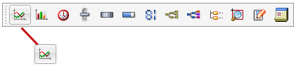
- Define the desired trend areaby dragging a rectangle on the panel area.
-
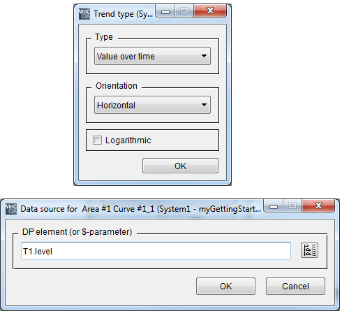
After releasing the mouse, the configuration dialog of the trend will be opened automatically. Confirm the first step of the dialog (Value over Time, horizontal, No "Log. Scales") with OK.
-
Enter the first curveT1.level in the dialog or select this data point using the data point selector. Confirm with OK.
-
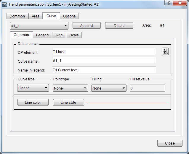
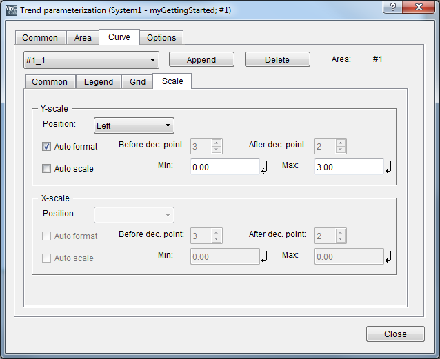
There are an inner and an outer level of tabs in the following dialog for configuring the trend. First the outer tab "Curve" will be opened and you can switch between the configured curves.
-
Click on Add next to the combo box in order to add a second trend line for the data point elementT2.level.The automatically added descriptions for the curves ( #1_2 forT2.level) only serve for internal processing. You will need these names for identification when using scripts. Moreover you can set the names.
-
Enter a fix scale of 0-3 m for T1.level and 0-1.4m for T2.level on the underlying tab. Note that you add the comma as "." (point).
-
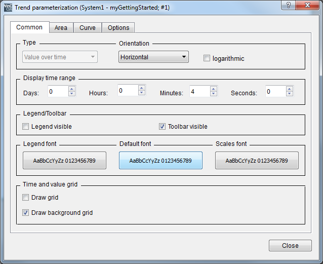
Switch to the outer tab "Common" and configure the following: for time interval increase the minutes to 4 and reduce the hours to 0.
-
Activate the check box "Legend visible".
-
Activate the check box "Drawbackground grid".
-
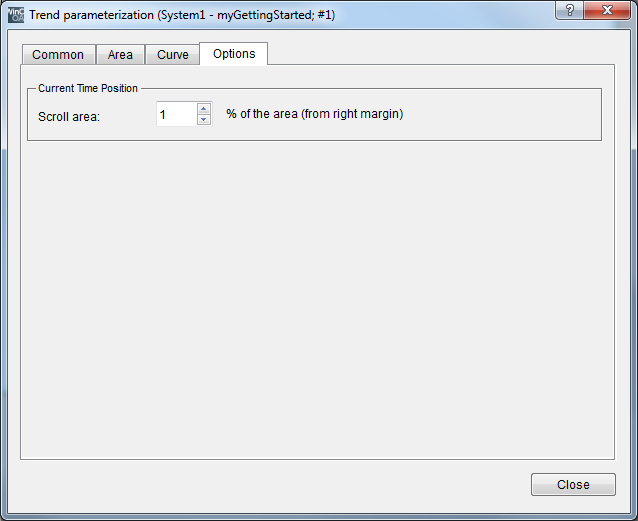
Switch to the outer tab "options" and enter 1% for the "image range". This setting specifies that the current time value is always located on the right side of the trend area and the maximum history will always remain visible. The curve will be moved to the left.
-
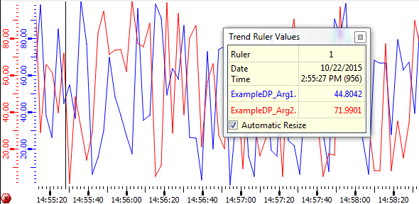
Finish the configuration and save the panel. Test the panel in the preview of the graphic editor. The view should correspond to the first figure on this page.
The trend line in the preview is first horizontally since the application does not possess a connection to the process. This will be changed as soon as you create a Simulation in the chapter 10.4. At the moment you can only change the curves by entering value changes in the PARA or (if configured) in Data point monitor for level displays.
For more information on the trend widgets, see chapters Trend or Bar trend. To use the trend through scripts, see chapter Trend functions.